Bifrost for Maya isn’t just an addition to the software; it’s a transformative tool that has been able to redefine the landscape of 3D animation, modelling and effects. With its advanced visual programming capabilities, Bifrost allows artists to push beyond the traditional boundaries and explore new creative horizons. The ability to manipulate strands, simulate lifelike fluids and fabrics, and perform complex calculations like the Material Point Method (MPM) within a single graph environment is a testament to the plugin’s power and flexibility.
The procedural modelling, rigging, animation and effects possibilities offered by Maya and Bifrost are virtually limitless (read our guide to the best animation software for more choice). The seamless integration with Arnold enhances this experience to provide a robust platform for rendering simulations with unparalleled detail and realism. The use of Arnold nodes within the Bifrost graph makes for a unified workflow that streamlines the creative process. Additionally, Bifrost’s comprehensive support for Universal Scene Description (USD) ensures compatibility within a broader production pipeline, particularly when used in conjunction with MayaUSD.
One of the pivotal features of Bifrost is the ability to output any command or process as a compound and publish it to make it available to other artists. For instance, in this project I used the powerful MJCG compounds, created by Maxime Jeanmougin, a fantastic Bifrost technical artist who’s currently collaborating with the Autodesk team on Bifrost’s development. This compound collection is available for free download at mjcg.gumroad.com and ready to be integrated into your own graphs.
Lighting plays a pivotal role in visual arts, setting the mood and atmosphere for the viewer’s experience. Without light, nothing can be seen, so spending time on it can help us share any feeling we choose with the audience.
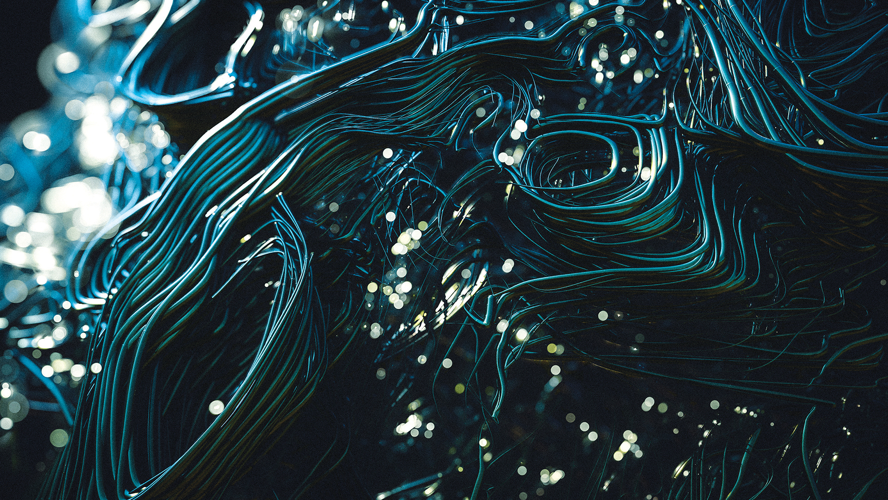
The core idea of this project was inspired by the remarkable artworks of Lee Griggs, who consistently creates ingenious and artistic visuals by blending the capabilities of XGen, Bifrost, and MASH. In this tutorial, we’ll aim to explore how we can craft a complex and robotic strand assembly using Bifrost’s strand creation feature, various fields, and Arnold nodes.
By setting up the camera and lighting in Arnold, we can capture outputs with different passes, and achieve a stunning final look with the help of the compositing software Nuke. Essentially, we’re looking to construct the final image in Nuke using a Z-depth pass to add cinematic depth of field and bokeh effects.
I used the latest version of Bifrost for this project, which you can download from the Autodesk website. However, you can tackle this project with earlier versions. If you like my tutorial then read Creative Bloq's Maya tutorials for more advice, and consider a new laptop for 3D modelling if you're serious about Maya and Bifrost.
01. Installing MJCG Compounds
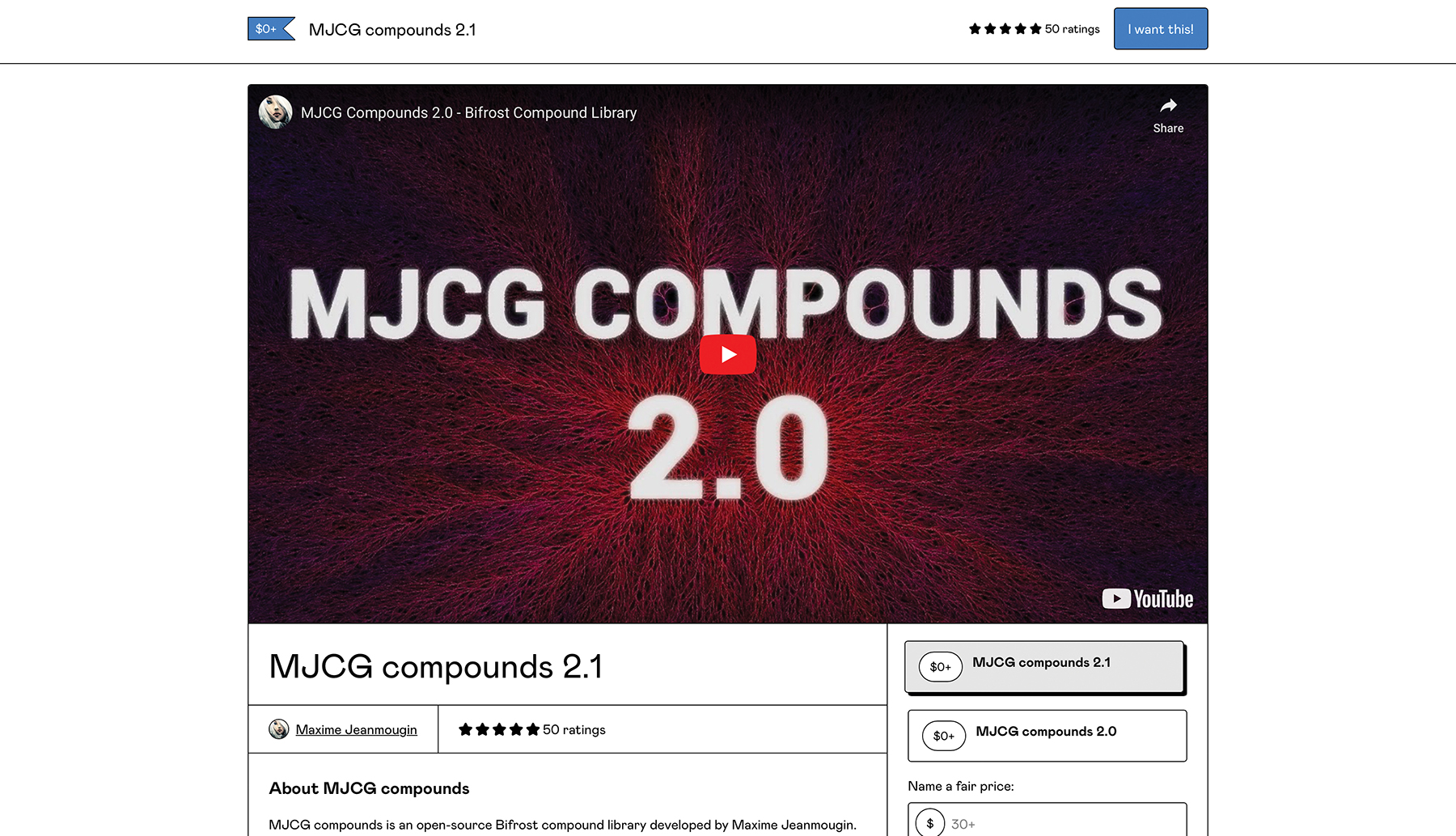
Before starting, we need to install the required compounds. Download the latest version of MJCG Compounds and copy it to a folder at the filepath ‘Users \ username \ Autodesk \ Bifrost \ Compounds’. If this address doesn’t exist, you can create the folders yourself. Do note that the latest version of MJCG Compounds works with Bifrost 2.6 and above. After copying, make sure to edit the ‘maya.env’ file and add this line of code to it:
BIFROST_LIB_CONFIG_FILES=C:/…/MJCG_compounds/bifrost_lib_config.json02. Opening the Bifrost Browser
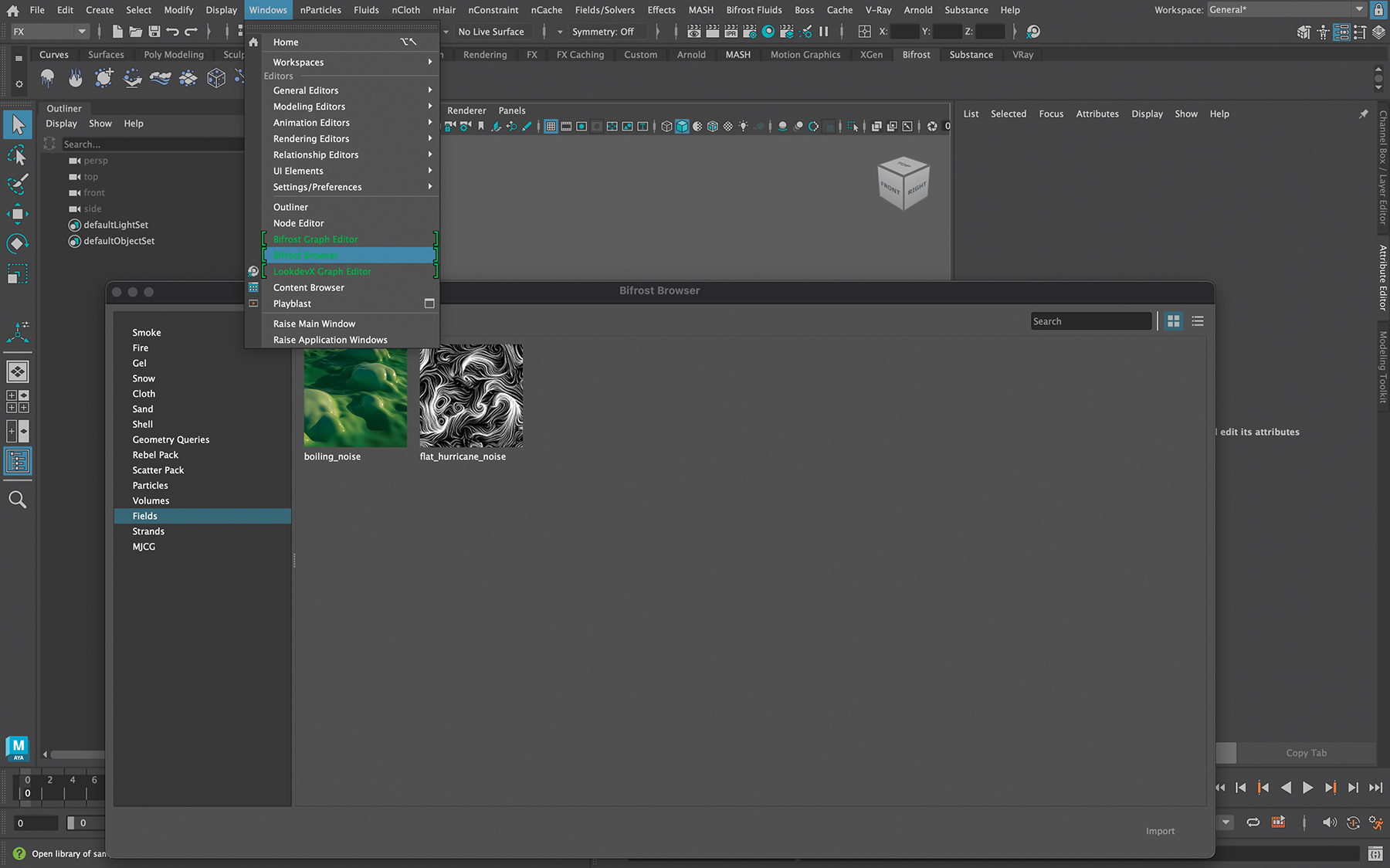
We want to open one of the default Bifrost scenes to create our own strands by changing the field parameters and setting input geometry. To do this, go to the Windows menu and select Bifrost Browser. There are numerous scenes you can explore by viewing the various graphs to see Bifrost’s capabilities. Click on the Fields section, select ‘flat_hurricane_noise’, and hit Import.
03. Using the Graph Editor intro
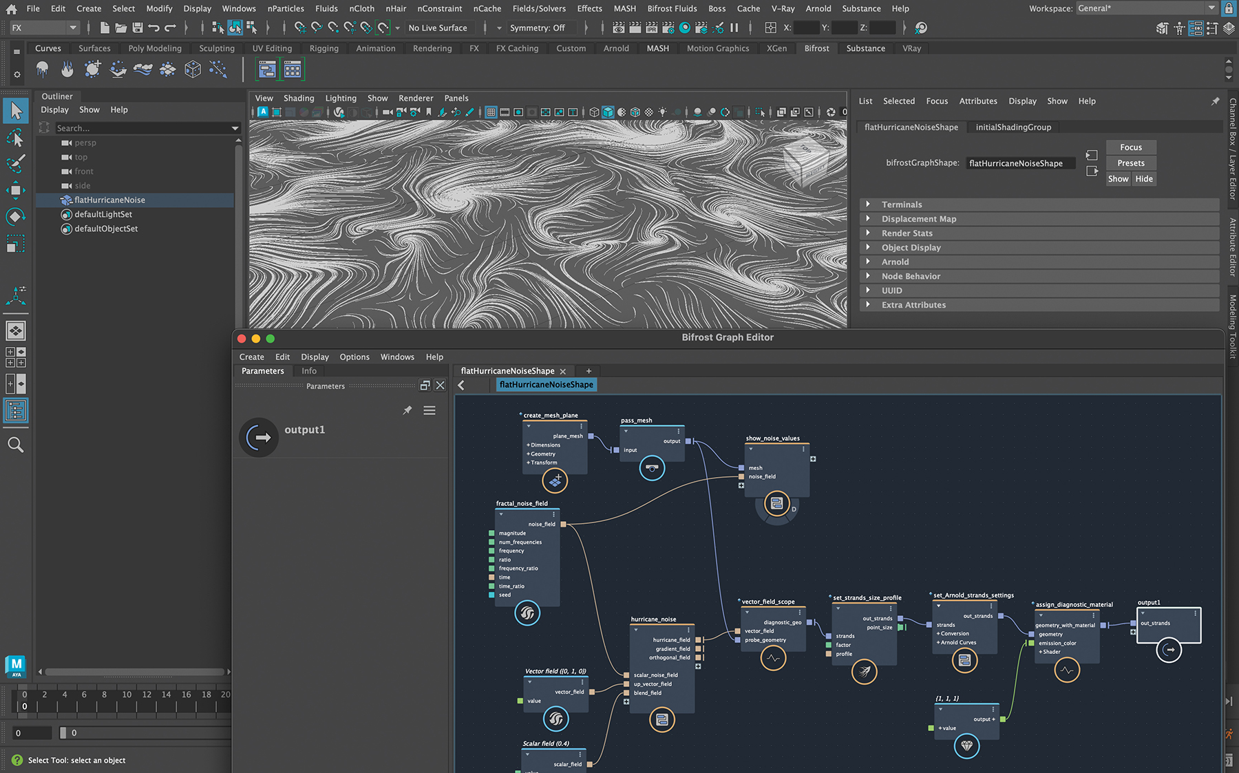
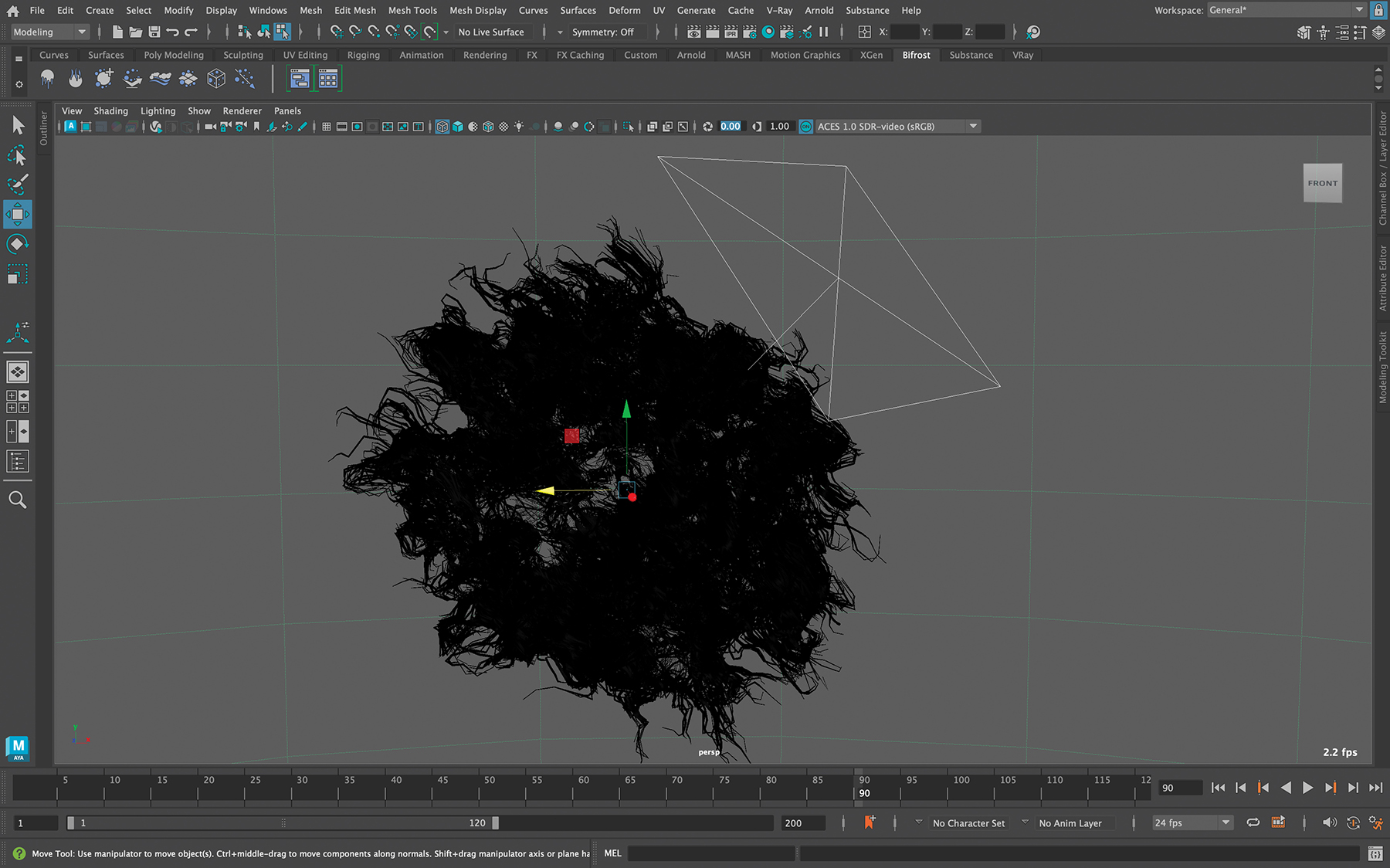
After the scene loads, go to Windows>Bifrost Graph Editor to see the nodes used in Bifrost. The result is a collection of twisted strands that have spread on the surface of a simple plane. This isn’t what we want, so we must change the shape of the strands by changing the base geometry, then control the appearance and number of them, and get the desired output using Arnold nodes.
04. Creating the base geometry
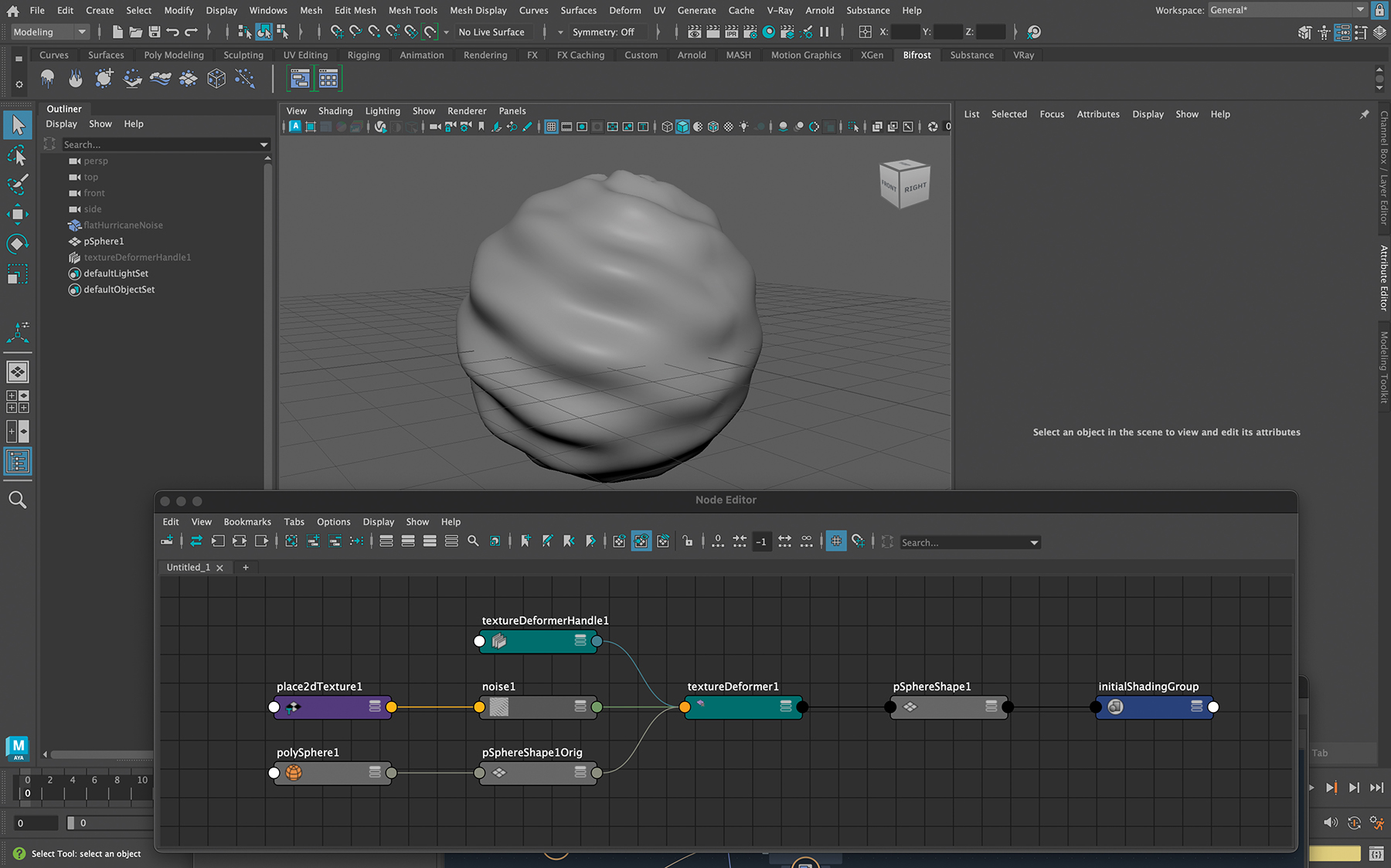
To manage the strands, we need base geometry. Create a sphere and increase the number of subdivisions. Next, select the Modeling menu set and open up the Deform menu. Add a Texture Deformer to the geometry, and within this node click the checker button to apply a texture input, choosing a 2D Noise node. Adjust the parameters to create any required shape.
05. Adding geometry to Bifrost
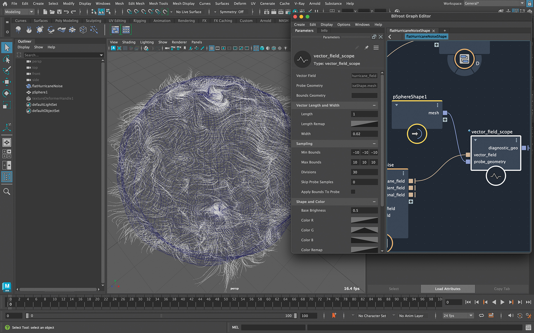
After creating the desired geometry, open the Outliner from the Windows menu, and drag and drop the selected geometry with a middle-mouse click. Once done, the newly added Geometry node should be visible in Bifrost. Next, connect the Mesh output from the Geometry node to the ‘probe_geometry’ input in the Vector Field Scope node. After this, you can see the changes to the strands in the Maya viewport. It will be evident that the strands are created on a sphere and no longer have a flat appearance.
06. Tweaking the strands
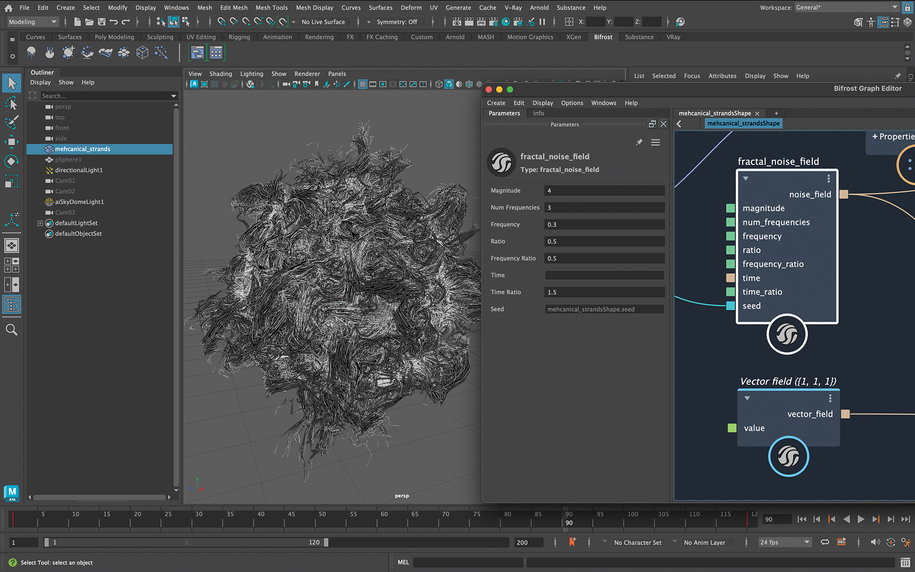
After connecting the base geometry, changes can be made with the Fractal Noise Field node and Vector Field values. By adjusting the Magnitude, Frequency and Ratio in the Fractal Noise Field, you can create twists and distortions. Once you’re satisfied, alter the impact on different axes with the Vector Field node connected up to a Hurricane Noise node.
07. Using the Curl Strands node
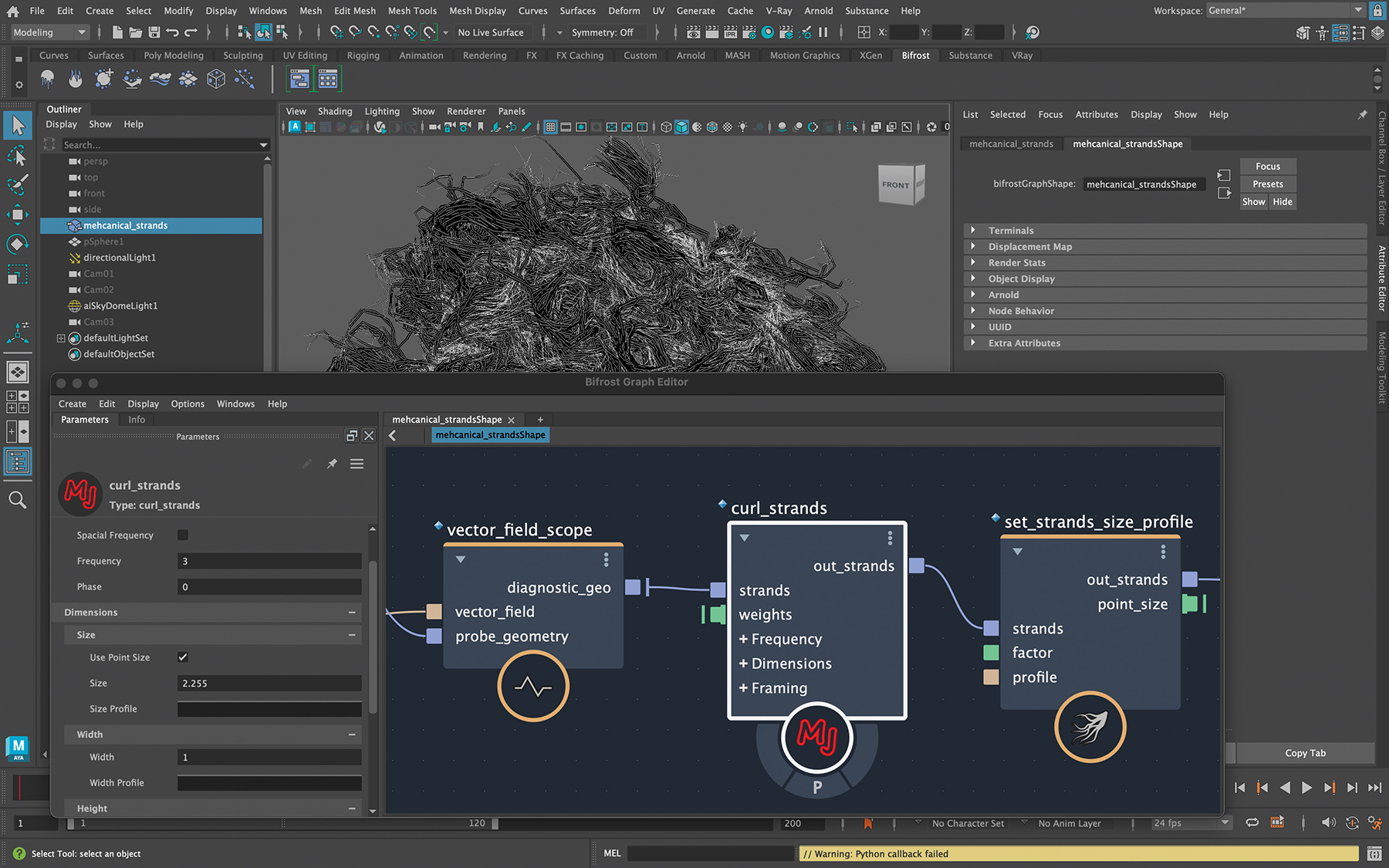
At this point we’ll find that we don’t have control over the twists and turns of the strands themselves after they’re generated. Here we can use a great node from MJCG Compounds called Curl Strands, which we’ll place between the Vector Field Scope and Set Strands Size Profile nodes. By changing the Size, Width and Frequency parameters, we can finalise the form of the strands.
08. Using Size Profile and Arnold Strands
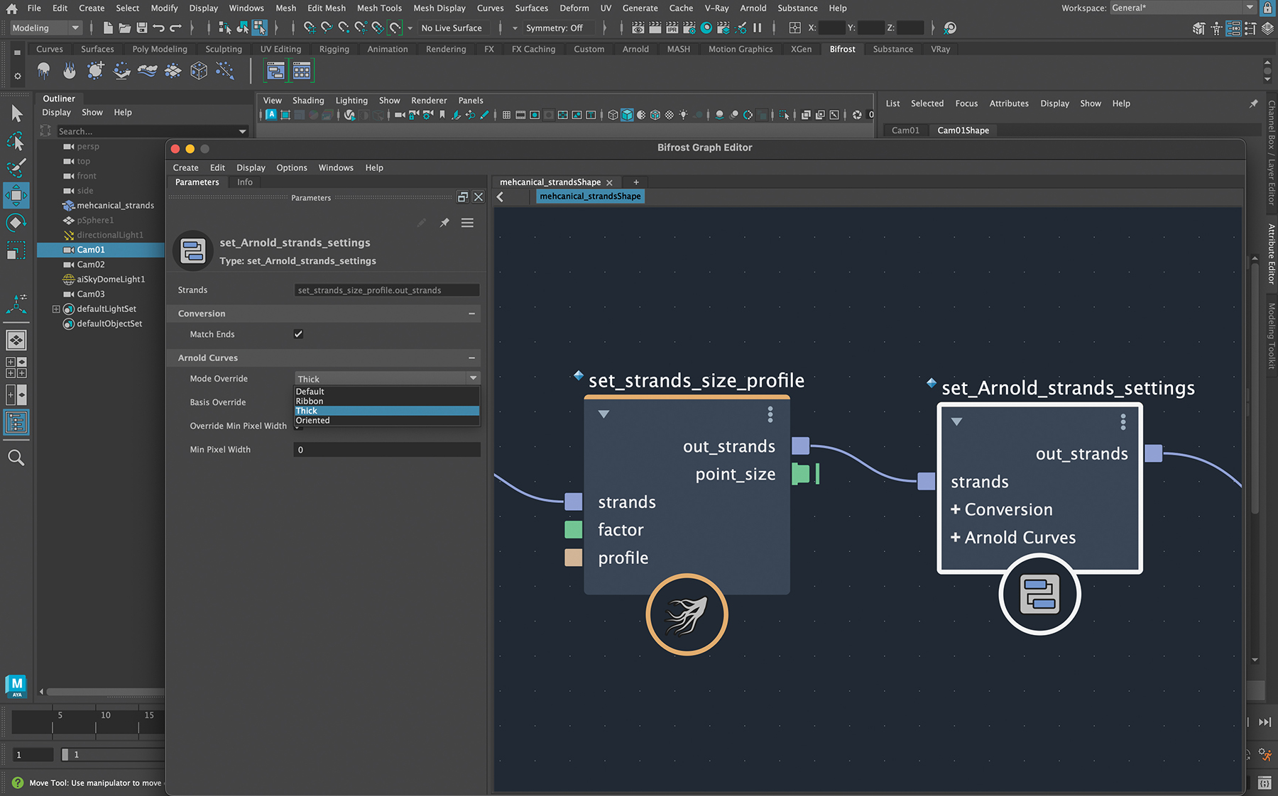
After setting the strands’ form, we can use the Set Arnold Strands Settings node to create their render shape in Arnold. The Mode Overrides option allows us to choose between Ribbon, Thick and Oriented for how the curves will appear during rendering. In the Set Strands Size Profile node, we can define the thickness of the curves with the Factor option and finalise it with Profile.
09. Setting-up the camera
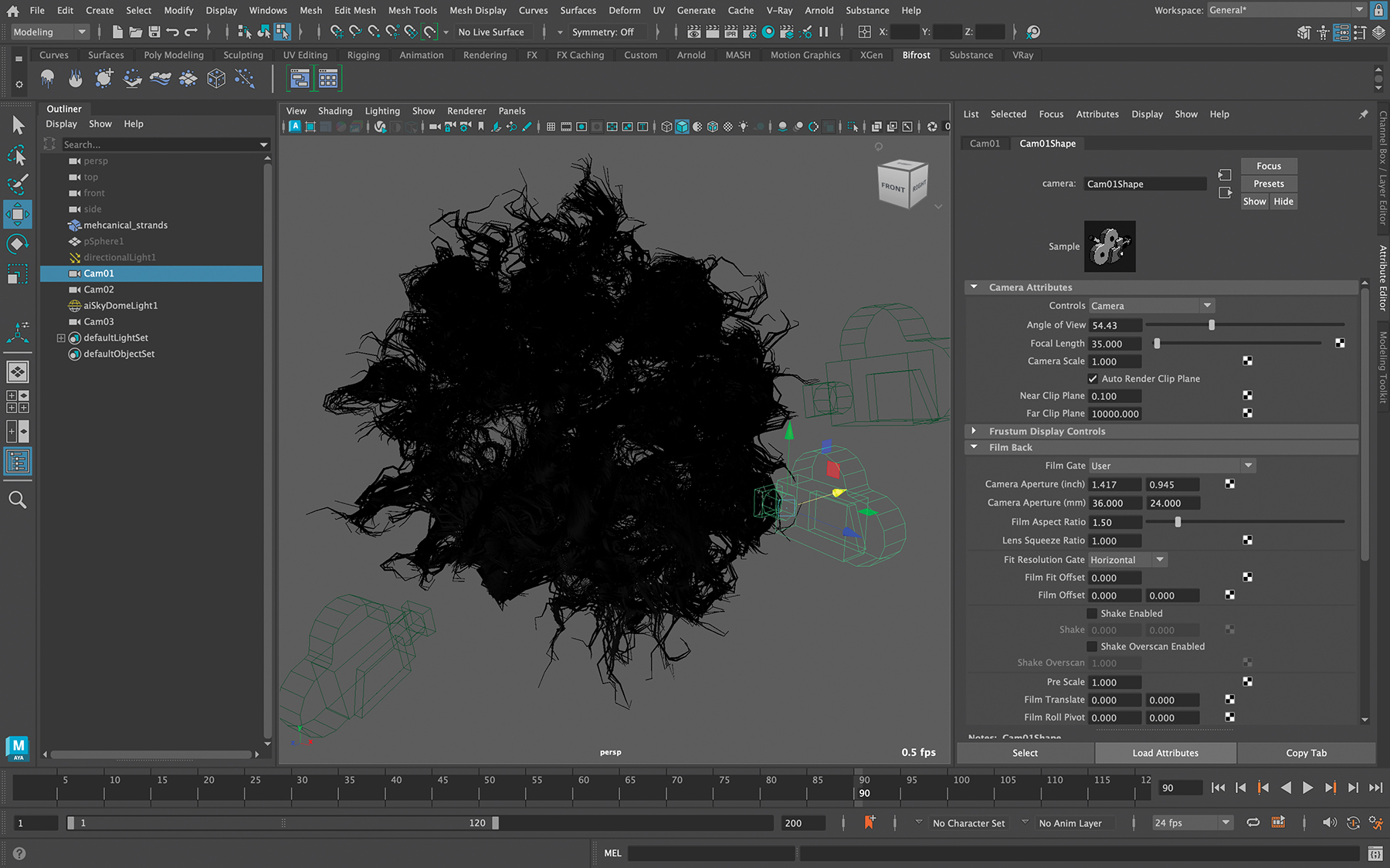
Camera angle, composition and lens selection are among the most important elements of a cinematic output. Each project requires considerable time dedicated to these aspects to achieve the desired result. It’s possible for several camera angles to be considered and advanced to the final stage before a definitive decision is made, and everything can be based on the final form of the strands. In this project, the final lens is 35mm with a low angle that precisely shows the main twists created by the Curl Strands node at the forefront of the image.
10. Making the material
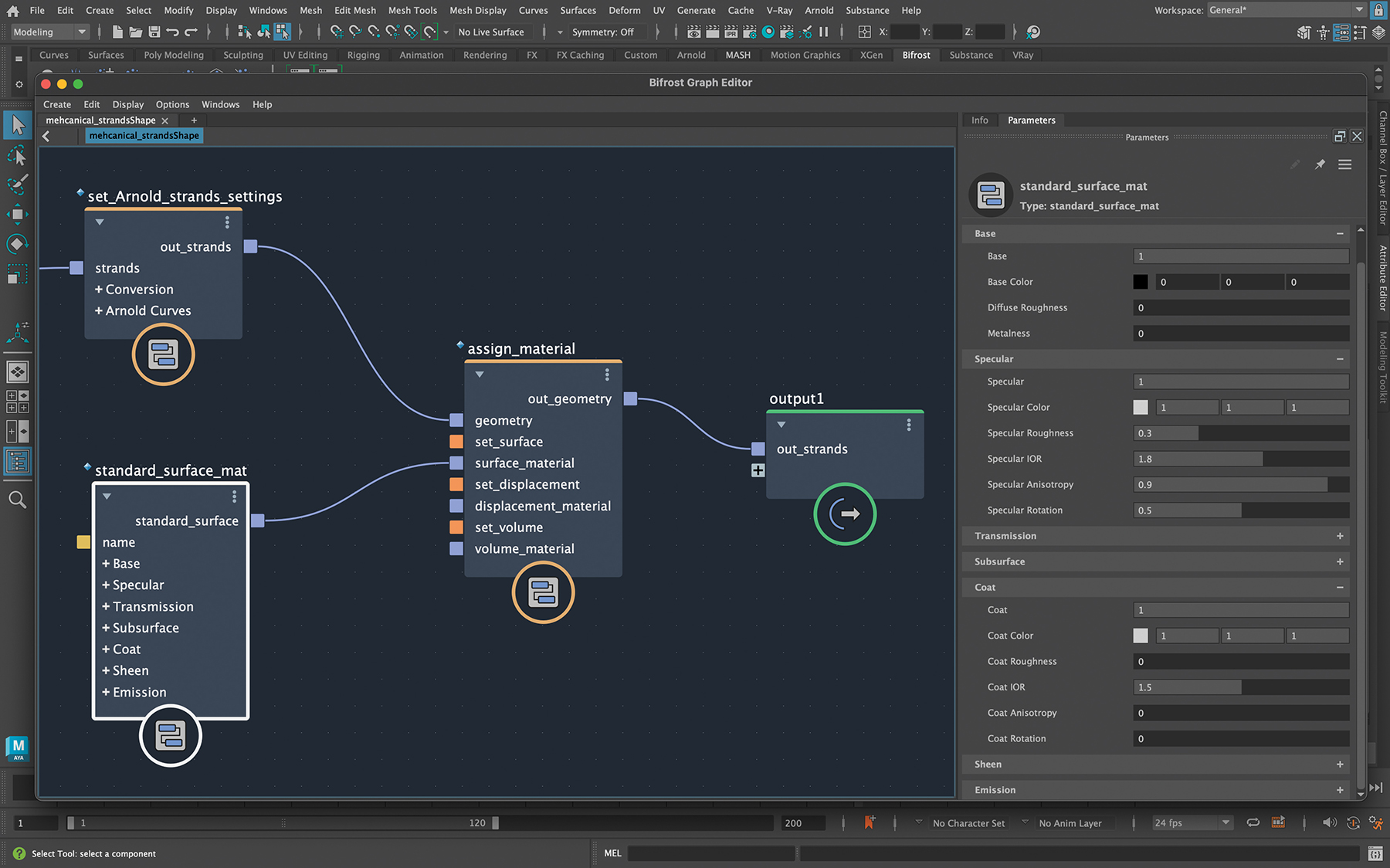
There are two possible methods for creating materials. The first is to make the material inside the Bifrost Graph by connecting the output of the Set Arnold Strands Settings node to the Geometry input of the Assign Material node. We then create a Standard Surface Material node and link its output to the Surface Material input of the Assign Material node. The other method is to select the output object of the graph in the Outliner, assign an AI Standard Surface material to it, and change the parameters in the Attribute Editor.
11. Setting-up the lighting
Let’s develop a dramatic and cinematic scene with lighting. We want the strands to appear mechanical and robotic, which needs sharp, intense reflections. Using an HDRI of an industrial factory filled with light can help create good shadows and highlights. Arnold lights such as area lights can also create reflections and speculars, setting us up for bokeh effects in the next steps.
12. Adjusting Arnold Standard Surface Parameters
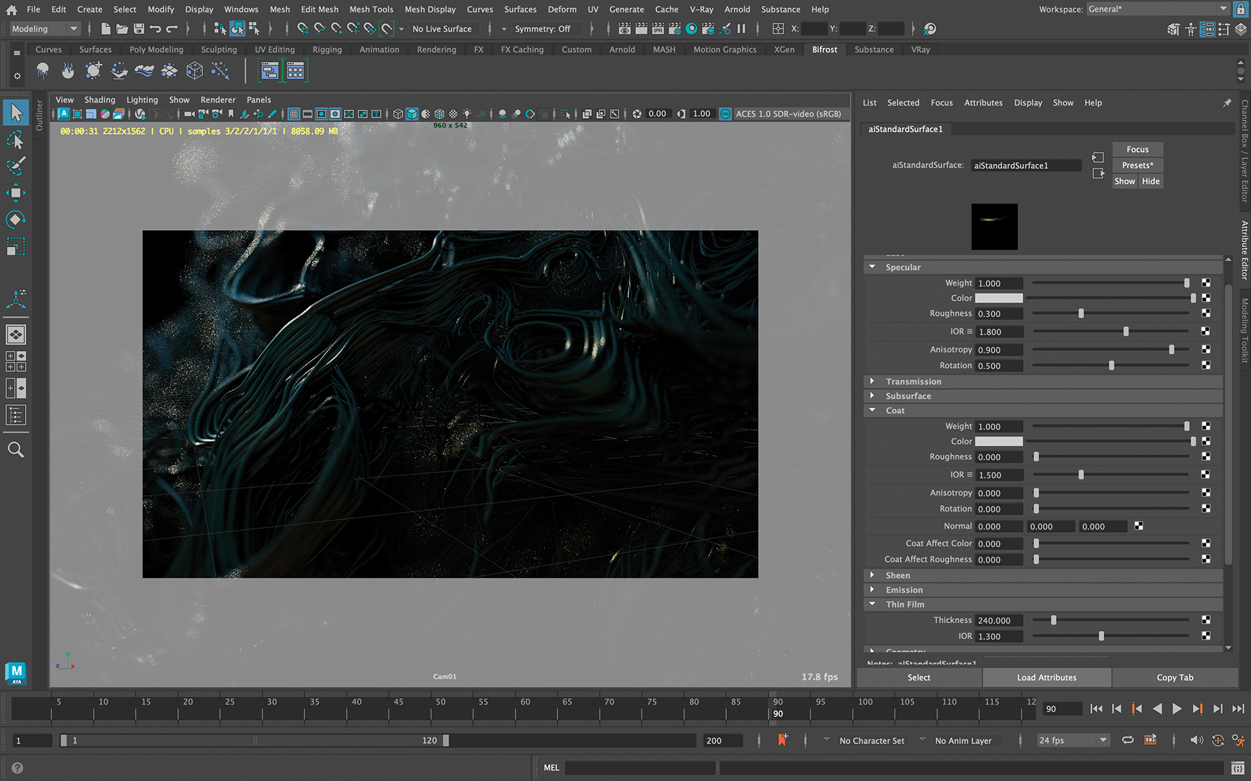
Lighting and material parameter adjustments are always a back-and-forth process. With lighting changes, you can also alter the material’s parameters. We want both matte and glossy reflections here, so make the Specular matte with a Roughness of 0.300. By changing the Anisotropy to 0.900 and Rotation to 0.500, we create elongated reflections. On top of this, set the Coat number to 1.000 for glossy reflections, adding a Thin Film with a Thickness of 240.000, and an IOR of 1.300, and change the Diffuse colour to black.
Lighting and rendering processes aren’t completely clear and defined before each project. While your experience in rendering can speed this up, it’s important to know it requires iteration and refinement to be executed in the best way possible.
13. Understanding Arbitrary Output Variables
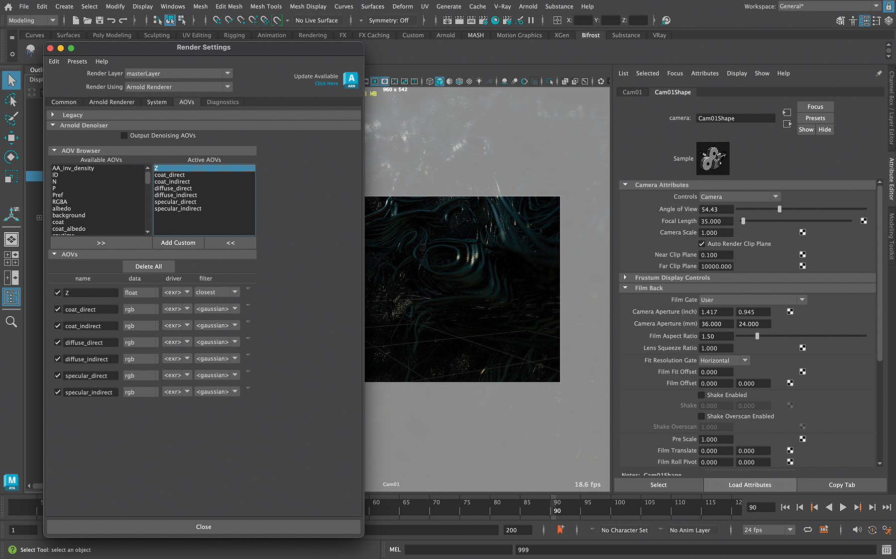
In the world of rendering, AOVs help us get different render elements separately so we can composite them as desired, and even add various effects. For example, using Specular and Reflection passes we can create a glow effect, or with Z-depth we can get depth of field in compositing. In this project, we want to output Z-depth, Specular, Diffuse and Coat passes.
Rendering each necessary element can give us complete freedom in compositing, allowing us to not only change the intensity of light, reflections and so on, but also to more easily solve any problems with the render.
14. Selecting Render Settings
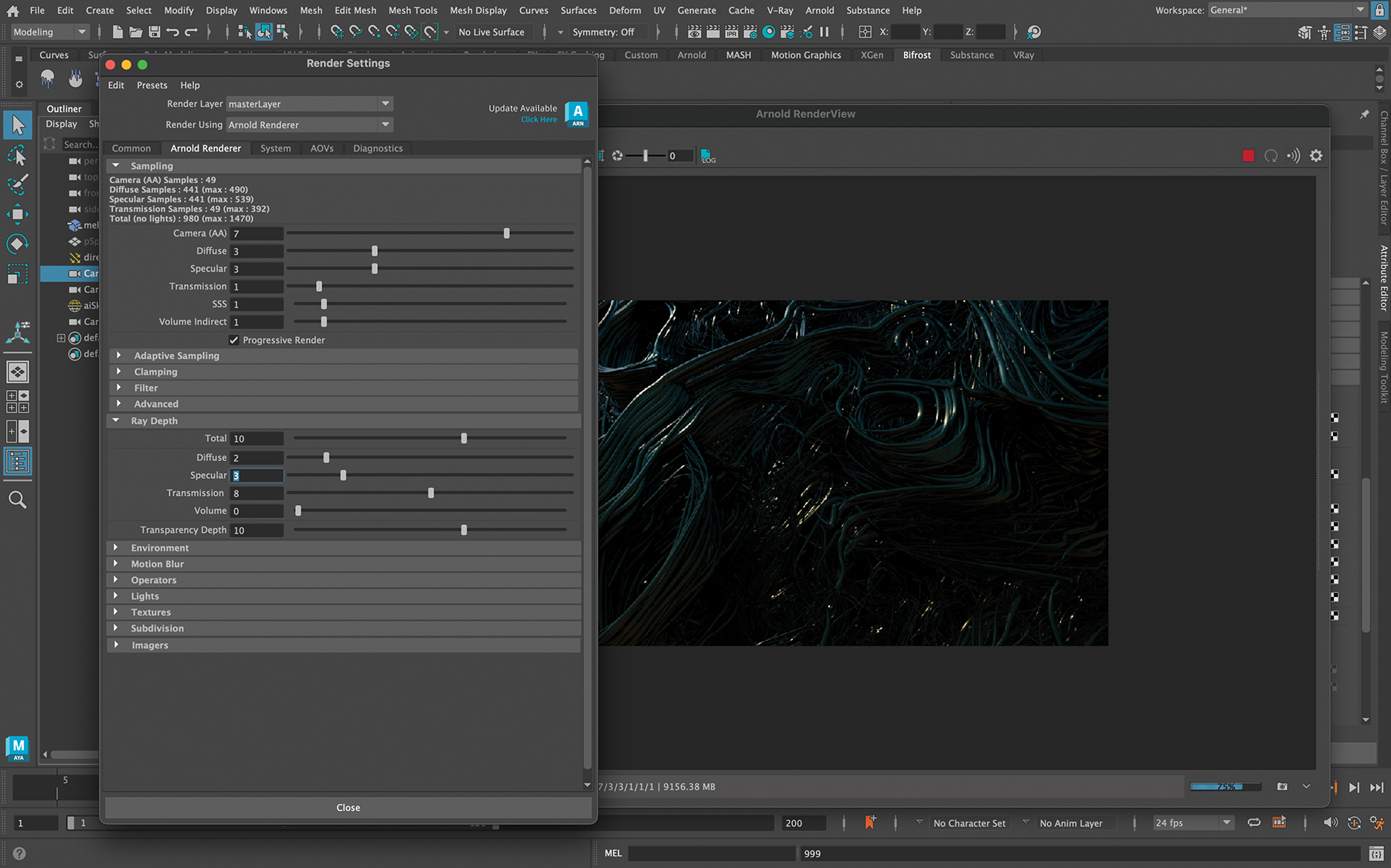
Sampling in render settings is key, and eliminating render noise hugely important. But remember that arbitrarily higher numbers means a longer render time. In this project, the sampling numbers were as follows: Camera AA 7, Diffuse 3, Specular 3. In the Ray Depth tab: Diffuse 2, Specular 3. Save the image as an EXR file and ensure all render layers are stored in the final image.
15. Using multi-pass compositing
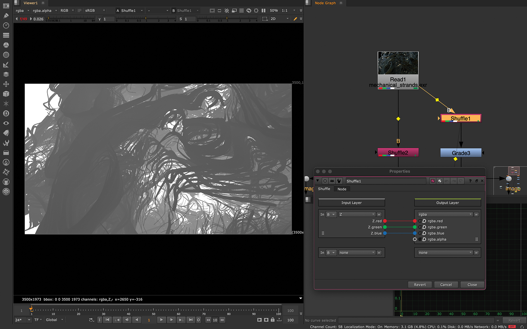
With Nuke, you have the ability to load an EXR file and use the Shuffle node to separate the individual render layers, then recombine them and change every layer as you want. You can also isolate the Z-depth pass to utilise its data with the ZDefocus node, which enables you to create your desired depth of field effect. This process hands you precise control over the final image by manipulating various individual elements and applying specific effects to enhance the resulting visual.
16. Adding Depth of Field
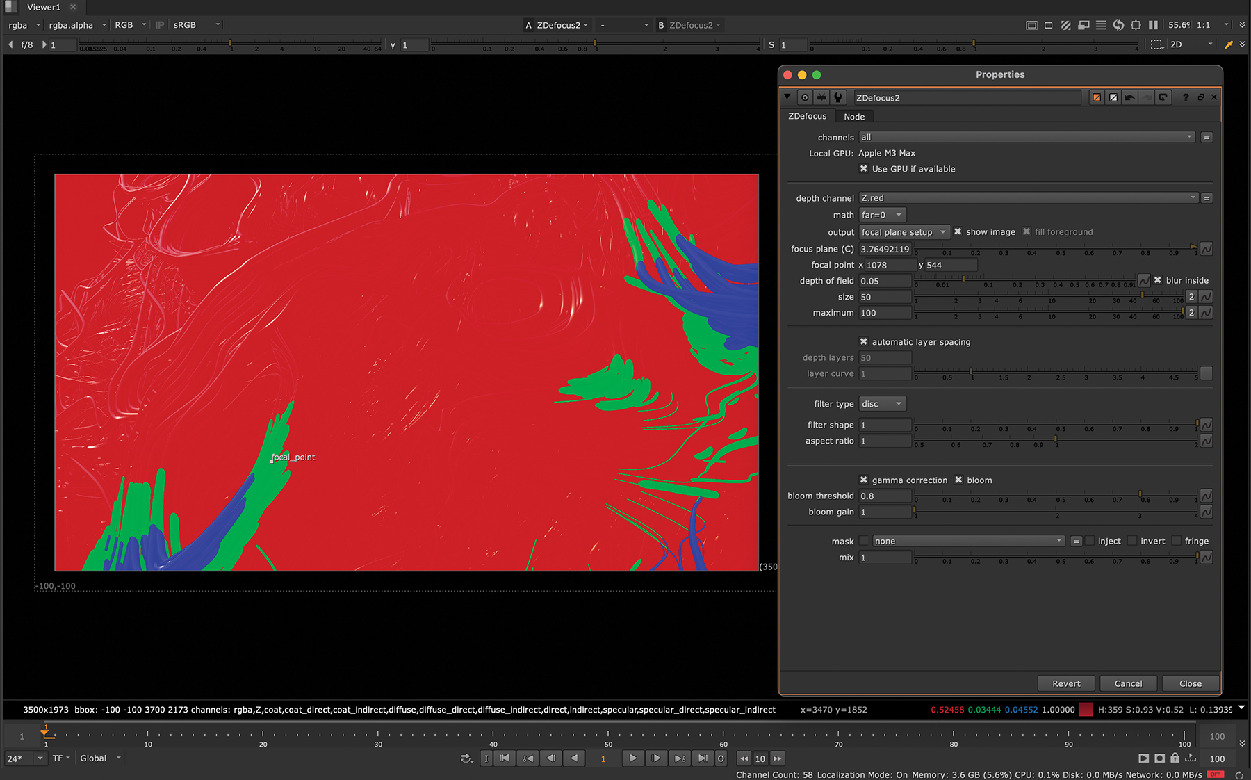
Next, let’s use depth of field and bokeh effects. Use the ZDefocus node and assign the Z-depth input to the Depth Channel. Now set the Output option to ‘focal plane setup’ and place the Focal Point where you want the focus to be. By setting the Size and Maximum, we can define the blurriness of the out-of-focus areas. For this project, we want to select ‘far=0’ as the Math algorithm.
17. Wrapping up the image
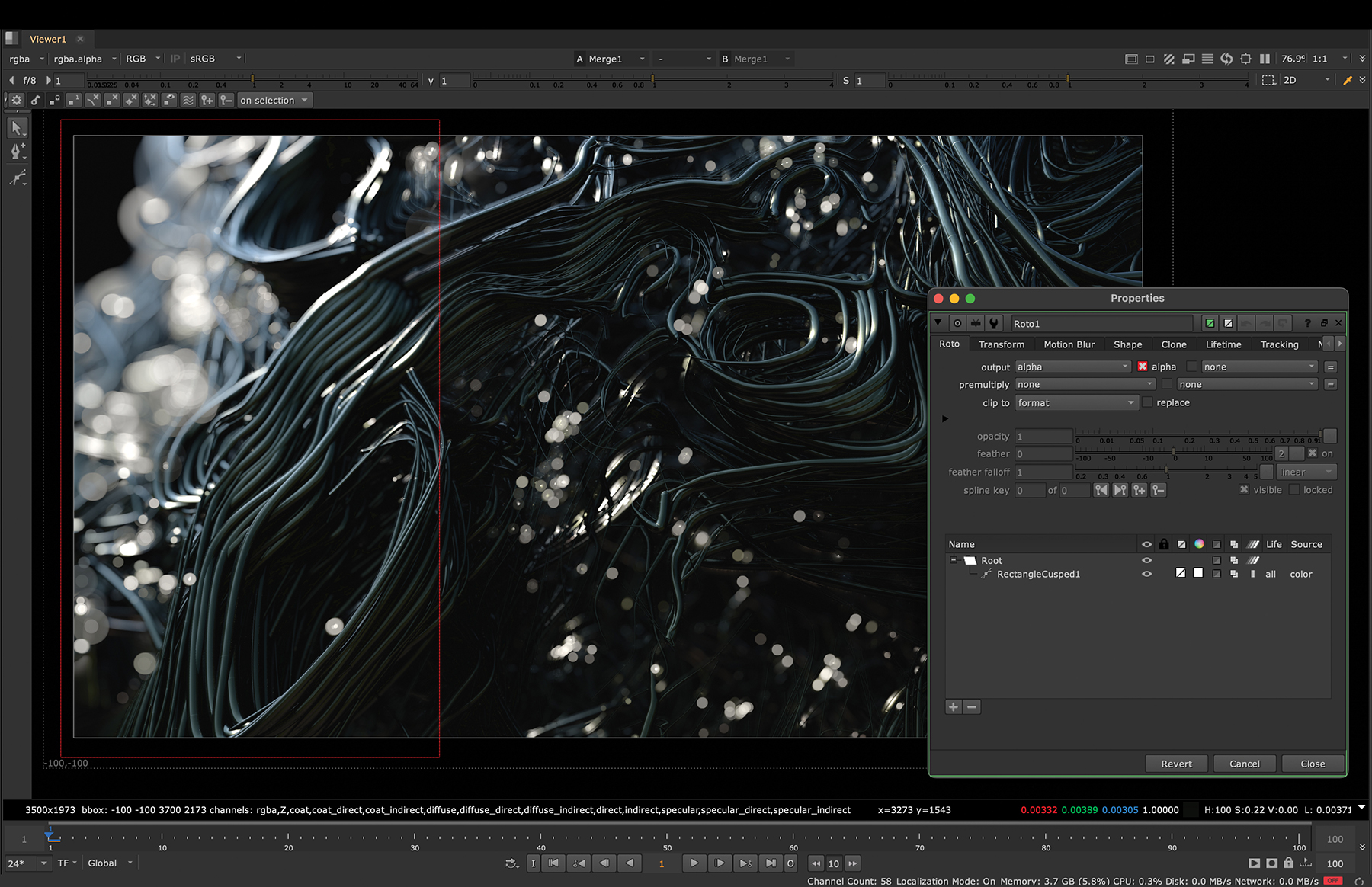
For the final image, we need two sections of depth of field, so we’ll use two setups and mask them with the Roto node. This way, we get larger bokeh effects in the back and left side of the image, and smaller bokeh effects on the front-right. Finally, the colours are corrected with Color Correct and Grade nodes, and a bit of noise and cinematic grain added with the Grain node.