How do you optimise for a Grand Tour time trial? The 2024 Giro d’Italia time trial course with 420 metres elevation gain is the perfect arena to delve into some time trial performance geekery. Our first challenge is to optimise our time with a cunning pacing strategy; then we’ll discover if a bike swap will be faster for the pros on Friday; and finally, will the stage be a day for a powerhouse like Filippo Ganna or a climber such as Tadej Pogačar?
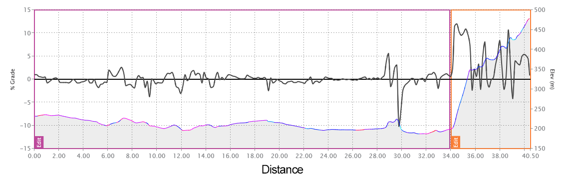
The interesting aspect of the 40.8km Giro time trial course is where the elevation gain is. The first 33km are comparatively flat. If the course was to end at kilometre 33, your best bet is to simply try to hold your highest sustainable power from Foligno to Ponte San Giovanni. However, our final destination is Perugia a further 7km uphill, with gradients peaking at 16%.
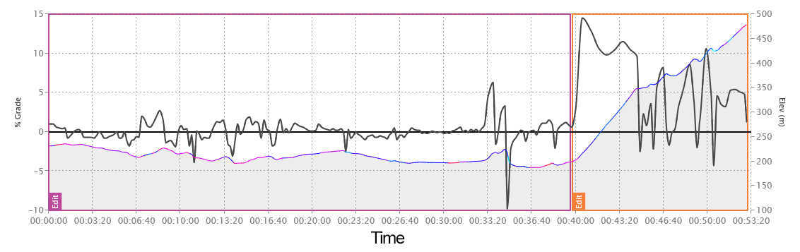
Below are two elevation charts. The first is the traditional elevation chart, with distance along the X-axis. The second chart shows a simulation time along the X-axis, revealing the significance of that final 7 km on the course.
Now to our challenge, optimising our power output for this course. Imagine we are a pro cyclist competing in the Giro d’Italia individual time trial. Our target power for the individual time trial is around 400 watts (~1300Kj). We choose to assign a conservative 20Kj additional 'budget' to optimise power strategy. I’ll explain why a budget would be decided this way shortly.
We can either:
- Evenly pace our time trial by spreading the kilojoules over the 40km
- Spend all our extra kilojoules on the final 7km uphill sector.
First of all, what is a kilojoule and why budget our energy this way and not in watts? A kilojoule is a measurement of energy. A watt is essentially one joule per second. So, to determine how many watts our 20Kj equates to, we must divide our kilojoules by the duration in seconds. By distributing energy rather than watts we can be sure we give each of our pacing plans a fair virtual race.
Watts = Kj*1000 / duration in seconds
Let’s begin by looking at how energy is distributed when cycling. This could give us a clue as to where our budget would be best spent.
First, we must contend with drivetrain losses. Anywhere two moving parts meet, there is a friction loss. The most efficient drivetrains are operating at 2% losses, whereas a standard well-maintained drivetrain will be around 3%. This means a rider cycling at 200 watts with a standard drivetrain has a net 194 watts contributing to the propulsion of the bicycle.
Next, I find it makes sense to split the remaining forces acting against us when we cycle into two categories, resistances affected by our mass (system weight) and Air Resistance. You’ll see why this is useful when I show you how the two behave differently as we change the velocity (speed) input in our formulas.
In our category ‘mass affecting resistances’, we have Gravity and Rolling Resistance. Cycling uphill obviously requires greater effort as we increase our mass due to gravity, but the sometimes overlooked effect of mass is on tyre rolling resistance.
Rolling resistance has a Coefficient. This is a ratio that describes how much force is required to overcome the vertical loading mass on the tyre. Typically a good road bike tyre is between 0.004 – 0.005. The higher the coefficient the greater the force required for the same velocity.
Take a look at how increasing mass affects both resistances.
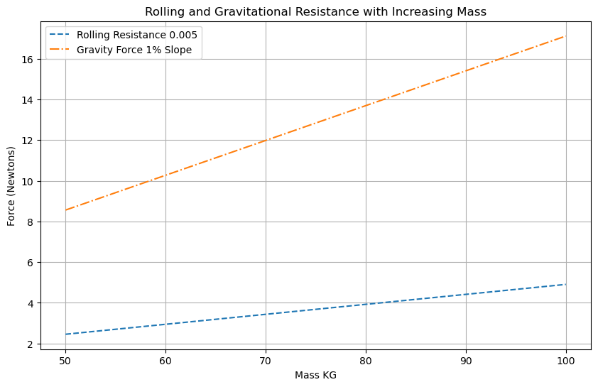
Rolling Watts = Rolling Coefficient * Gravity * Mass * Velocity
Equation for Rolling Resistance
Gravity Watts = Mass* Gravity * sin(Slope) * Velocity
Equation for Gravitational ‘Resistance’
Air Resistance is what we call an exponential force. The next chart shows how Air Resistance responds to our Speed increasing. Notice how it wouldn’t be easy to draw this line with a ruler.
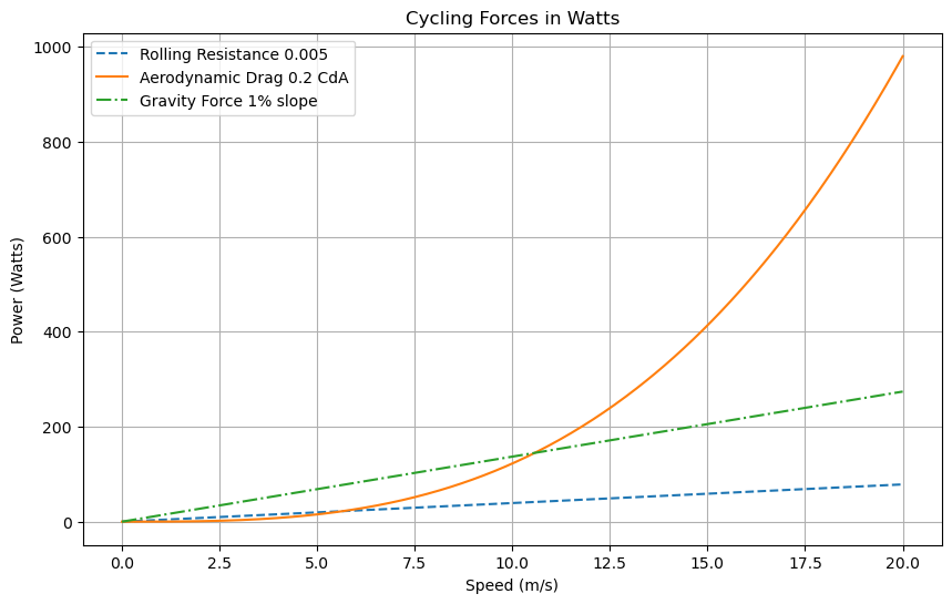
Air Resistance gets out of hand very quickly compared to our linear mass affected resistances.
The inputs for Air Resistance is Air Speed, Air Density, and our Coefficient of Drag (CdA). Notice we are using Air Speed and not Ground Speed.
Air Watts = 0.5 * Air Density (rho) * CdA * Air Speed2 * Velocity
Equation for Air Resistance
So, there’s a very quick run-through of the resistances we must overcome to cycle faster. Now back to our time trial challenge.
As we aren’t using a supercomputer such as myWindsock.com to process every metre of our time trial including the weather, we’ll need to simplify our course into two sections, a 33km 0% gradient sector and a 7km sector with an average gradient of 4.5%.
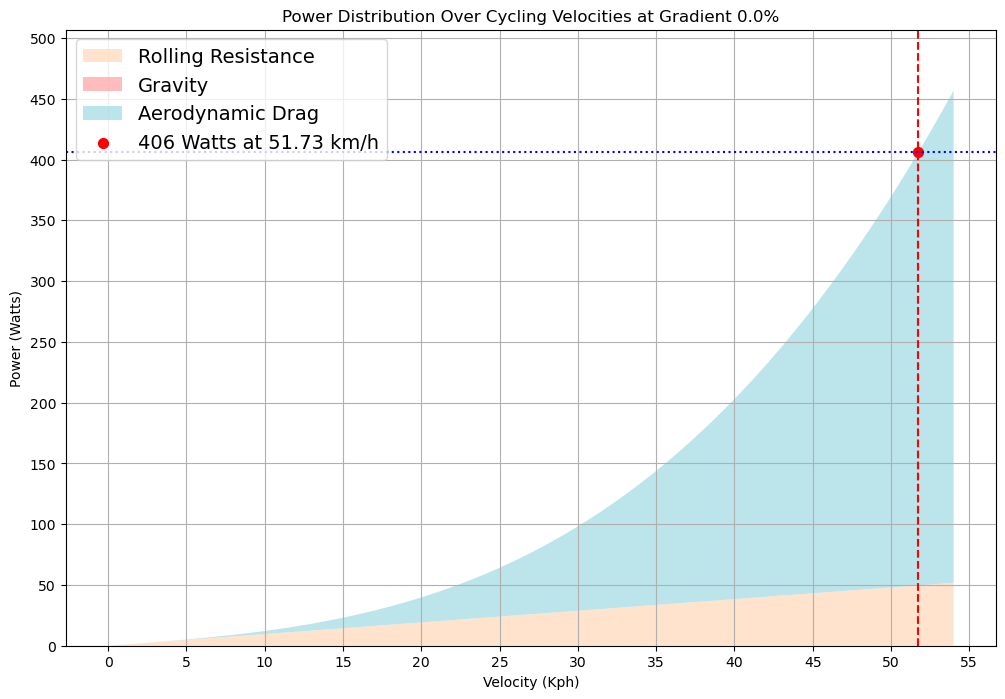
So far our formulas give us the required power to overcome resistance at a given velocity. Our pacing experiment requires us to determine Velocity (speed). Now this gets tricky as you’ll notice we require Velocity in both our linear and exponential (quadratic) equations. In order to solve our linear equations we need the answer to our exponential equation and vice-versa. To solve this, plotting on a chart comes in handy.
Below are our charts to solve our initial estimates of time duration. We’ll start with a baseline duration for both the 33km flat sector and the final 7km uphill sector. We are doing this so we are able to fairly distribute our 20Kj budget in our two scenarios over the estimated time duration.
For the following calculations we have a CdA of 0.2, rolling resistance of 0.0044 and our system weight (mass) is 80kg.


Using the above graphs, we have located our speed estimates. To get our durations for each section, we must divide speed over distance.
Now, we calculate our additional wattage for our evenly paced time trial. Dividing our 20Kj over the total baseline time of 52:13 gives us an additional 6 watts. 52:13 equates to 3133 seconds, and 20Kj (or 20,000 joules) divided by 3133 equals 6.38 joules per second. For simplicity, we've rounded down to 6 joules per second, which equates to 6 watts.
Using the formulas discussed earlier let’s generate our graphs another time. This time with our power set for an evenly paced time trial at 406 watts (original 400 plus 6 watt extra 'budget')
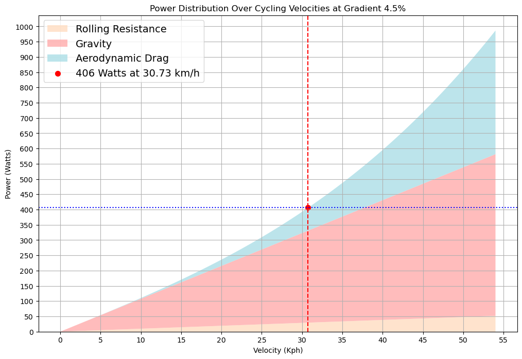
Again we calculate our total time in the same way.
The additional wattage has gained us 18 seconds. This is unsurprising given we’re 6 watts up on baseline power. However, did you notice the relative change of our speeds was much greater for our final uphill 7km?
Now for our 20Kj budget to be deployed only in the final 7km uphill sector. We revert back to our initial estimated time of 13:47 and divide our 20Kj. This gives us 24 extra watts, taking us up to 424 watts for the climb. We already know the time of our first 33km at 400 watts was 38 minutes 26 seconds. But, what will our final 7km be? Let’s run the maths and look at the graph.

One last time, we calculate our total time in the same way.
For the same energy expenditure, we gained a further 15 seconds simply by distributing it differently. In fact, it would be more than this due to the fact that we have shortened our sector time, meaning we could potentially output even more power and be even quicker. To perfectly match Kilojoules, we would again need to perform multiple iterations to get within our acceptable margin of error.
Of course, the actual Giro course has varying gradients. As the gradient increases, the effectiveness of our additional power will increase.
Why are we quicker when applying our extra power to the uphill sector? Let’s refer back to those linear and exponential equations. As air resistance increases our return for each watt becomes less and less, as demonstrated by the exponential curve. Whereas the linear forces, gravity and rolling resistance, have a much more favourable input-to-output return.
Looking forward to stage 7 of the Giro, what does our time trial geekery reveal? For the following insights, we must factor all the twists and turns, inclines and declines and the evolving weather.
To do this, I reach for the AI-powered simulator, myWindsock.com.
Would a bike swap make sense?
We’ve already explored the fact that in the final 7km to Perugia has an average 4.5% gradient. But, that only tells half the story. For the first 1.5km the road averages 10%, peaking at 16%. At those grades, we could be in the territory of a bike swap. The basic requirement of the math here is to work out whether the reduced weight of the road bike when compared to the time trial bike makes enough difference to the rider's speed to offset the aerodynamic detriment plus the time it takes to stop and swap. To work this out, we'll do the sum for two riders: heavyweight Filippo Ganna and lightweight Tadej Pogačar, but we also have to make some assumptions.
For our simulations, we’ll assume the road bike available is around 2kg lighter than the aero bike and both riders are riding at their reported FTPs (Functional Threshold Power), and we'll use the weight reported by ProCyclingStats. We'll also assume a fixed CdA for both bikes/riders.
So a few seconds lost between swapping bikes could leave a small advantage. The simulated advantage may be smaller than you’d expect, but our simulation also takes into account the reduction of ‘potential energy’ due to the smaller mass.
To demonstrate potential energy, would you rather be hit by a train or a feather travelling at 30kph?
Digging deeper, if we factor in aerodynamic losses we find that the road bike will put the rider at an overall disadvantage, especially after the first 1.5km have been climbed and the road levels off some. We can quickly simulate this to find out.
Assuming our rider on a road bike has a fixed CdA of 0.3, whereas above 20Kph (ie, after the initial section of the climb) our time trial bike will return to a slippery CdA of 0.2.
In this sum, the road bike is half a minute down on the TT bike setup, so a bike swap wouldn’t make sense. However, teams will know more accurately the CdA, weight and power outputs for each of their riders on both road and time trial setups, as well as how quickly they can swap from one bike to another. If the CdA detriment is smaller, or the weight difference is greater, then it might swing things in favour of a bike swap, assuming they can get it done quickly!
Can a heavyweight like Ganna hold off a lightweight like Pogačar?
This takes a bit of guesswork as to the power outputs on the day. However, we can see that this course will beautifully expose the strengths and weaknesses of both types of rider. Assuming both are riding at their reported FTPs, we can see how close this could get with a time delta graph. Below shows a simulated time comparison between Ganna and Pogačar.
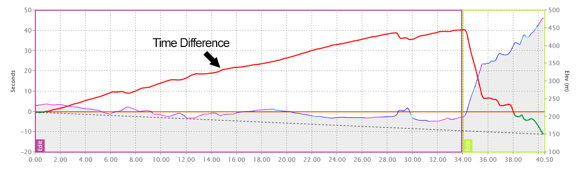
The red line shows Ganna taking time out of Pogačar up to time checkpoint 2. In the final sector, Ganna is quickly losing his advantage. For Ganna to be in contention, he needs to lead Pogačar by more than 50 seconds at time check 2.
As we learned earlier, it will pay for both riders to 'negative split' the race, saving some joules on the flat ground before setting the matchbook alight on the climb. It might just be tough for the lighter riders to accept the time deficit at the first checkpoints and believe that the math will come good in the end.
It’s certainly going to be one to watch.